PointNet
Point cloud는 정해진 format이 존재하지 않아서 기존 연구는 image들의 집합으로 바꾸거나 3D voxel grid로 집어넣었지만, 본논문은 point cloud 자체를 input으로 넣음 -> permutation, rigid motion invariant 해야함
point cloud feature를 잡기위해서는 어떻게 해야될까?
전통적으로 통계를 이용하여 특정 변환에 invariant하게 encode 했고 이 종류에는 intrinsic,extrinsic이 있고 local features인지 global features인지도 갈린다.
- Deep learning on 3D data:
- Volumetric CNN: voxelize 한 point cloud에 3D convolutional neural network를 적용 했지만, volumetric representation은 data sparsity와 3d conv의 연산량 때문에 비효율적
- FPNN, Vote3D : sparsity를 개선하고자 나온연구이지만, 여전히 sparse한 volume을 가지고 있었다.
- Multi-view CNN : 3D point를 2D image 로 렌더링 하고, 2D conv net을 적용하였다. shape classification같은 검색 task에는 잘됐지만 scene understanding이나 3D task에서는 주도적이 아니었음
- Spectral CNN , Feature based DNN 등 최신 연구들(그 당시에)은 mesh(3차원물체) 에 spectral CNN을 적용하였다. 그러나 이것은 organic objects 에 제약이 있었고(Spectral CNN), 첫번째로 3D data를 vector로 전환하였고 fully connected net 을 classfication에 적용하였고 이것은 추출된 특징점들의 표현에 제약이 있었다고 생각한다( feature based DNN) 추후 필요시 공부 예정

아래 보는 것 처럼  point를 이미지화 해서 cnn에 집어넣는 것은 작동하지만 가장 큰 문제는 cubic voxel grid of size 100가 1,000,000 voxels을 가지게 될 것임 - 매우 큰 낭비 / Mult-view CNN의 예
input : point cloud (x,y,z) 원래는 color 같은 알파도 있지만 편의상 제거 output : object classification : k class 후보에 대한 k score ,segmentation labelsemantic segmentation n*m score (n points and each of the m semantic subcategories 에대한)
3. Problem Statement
3d point data 특성 3가지 : unordered, invariance under transformation(변환에 불변), Neighborhood points 간의 연관성
PointNet Architecture

Symmetry Function for Unordered Input
f(x, y, z)=f(y, z, x)를 만족하는 것이 symmetry function
permutation invariant 하기 위해서는 기존에 사용하던 방법이 성능이 좋지않아 부가적인 Maxpooling layer를 사용
(point 마다 mlp를 통해 1024개의 feature를 생성하고 각 점 마다 1024개의 feature를 만들어 nx1024가 되면 column-wise maxpooling을 통해 1024개의 output이 나오게함) -> 추후 Joint alignment Network 코드에 예시 있음
이때, mlp의 weight는 모든 점들마다 동일하게 사용(weight sharing)
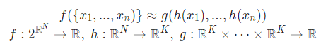
h : multi-layer perceptron network, g : max pooling function
Local and Global information Aggregation
segmentation을 위한 부가적인 네트워크 / segmentation은 local&global 정보가 모두 필요하므로 global feature vector를 계산하고 나서, 각 point feature 에 이 global feature를 붙혀 새로운 point feature를 얻는다.
Joint alignment Network

회전,이동 같은 rigid transformation 에 의해 semantic labeling 결과가 변화하면 안되서 본 논문에서는 T-net 구조를 2개 사용하여 affine transform을 수행하였다. -> 다른 input point clouds 를 정렬시키기 위해서(architecture의 T-Net)
(흥미롭게도, 우리는 3D space안의 translations을 3dim matrix로 encode할 수 없다.)
어쨋든, Tnet구조를 살펴보면 STN(spatial transformer network)과 유사하다. 사진을 보면 mini pointNet이 구성되어 있고 T-net에서 Point data를 canonical space로 보내기위한 transformation matrix를 계산하고 input data에 transformation matrix를 곱한다.
STN 이란?
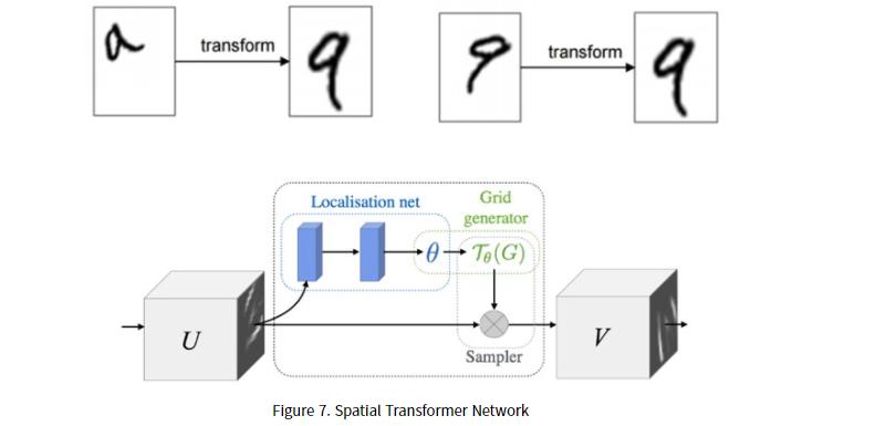
input transform에 비해 feature transform의 차이점이라곤 규제항 추가이다.
feature transform이 spatial transform보다 훨씬 높은 차원이라 optimization이 어려워 규제항을 추가함 (spatial transform은 일반적인 공간 변환을 말하는 거 같음)

Tnet의 구조는 다음과 같다.
import torch
import torch.nn as nn
import torch.nn.functional as F

class Tnet(nn.Module):
   def __init__(self, k=3):
      super().__init__()
      self.k=k
      self.conv1 = nn.Conv1d(k,64,1)
      self.conv2 = nn.Conv1d(64,128,1)
      self.conv3 = nn.Conv1d(128,1024,1)
      self.fc1 = nn.Linear(1024,512)
      self.fc2 = nn.Linear(512,256)
      self.fc3 = nn.Linear(256,k*k)

      self.bn1 = nn.BatchNorm1d(64)
      self.bn2 = nn.BatchNorm1d(128)
      self.bn3 = nn.BatchNorm1d(1024)
      self.bn4 = nn.BatchNorm1d(512)
      self.bn5 = nn.BatchNorm1d(256)


   def forward(self, input):
      # input.shape == (bs,n,3)
      bs = input.size(0)
      xb = F.relu(self.bn1(self.conv1(input)))
      xb = F.relu(self.bn2(self.conv2(xb)))
      xb = F.relu(self.bn3(self.conv3(xb)))
      pool = nn.MaxPool1d(xb.size(-1))(xb)
      flat = nn.Flatten(1)(pool)
      xb = F.relu(self.bn4(self.fc1(flat)))
      xb = F.relu(self.bn5(self.fc2(xb)))

      # initialize as identity
      init = torch.eye(self.k, requires_grad=True).repeat(bs,1,1)
      if xb.is_cuda:
        init=init.cuda()
      '''C. Network Architecture and Training Details(Sec 5.1)
      이 부분에서 training할 때, 어떠한 transformation도 없는 상태에서 시작하길원해 출력에 항등
      행렬을 추가함
      add identity to the output'''
      matrix = self.fc3(xb).view(-1,self.k,self.k) + init
      return matrix
Transform의 코드는 다음과 같다.
class Transform(nn.Module):
   def __init__(self):
        super().__init__()
        self.input_transform = Tnet(k=3)
        self.feature_transform = Tnet(k=64)
        self.conv1 = nn.Conv1d(3,64,1)

        self.conv2 = nn.Conv1d(64,128,1)
        self.conv3 = nn.Conv1d(128,1024,1)

        self.bn1 = nn.BatchNorm1d(64)
        self.bn2 = nn.BatchNorm1d(128)
        self.bn3 = nn.BatchNorm1d(1024)

   def forward(self, input):
        matrix3x3 = self.input_transform(input)
        # batch matrix multiplication
        xb = torch.bmm(torch.transpose(input,1,2), matrix3x3).transpose(1,2)
        xb = F.relu(self.bn1(self.conv1(xb)))

        matrix64x64 = self.feature_transform(xb)
        xb = torch.bmm(torch.transpose(xb,1,2), matrix64x64).transpose(1,2)

        xb = F.relu(self.bn2(self.conv2(xb)))
        xb = self.bn3(self.conv3(xb))
        xb = nn.MaxPool1d(xb.size(-1))(xb)
        output = nn.Flatten(1)(xb)
        return output, matrix3x3, matrix64x64
loss fuction에서 아까 말했던 regularization term을 추가한 것을 볼수 있다. 따라서 (AA^T = 1) orthogonal에 가까워진다.
def pointnetloss(outputs, labels, m3x3, m64x64, alpha = 0.0001):
    criterion = torch.nn.NLLLoss()
    bs = outputs.size(0)
    id3x3 = torch.eye(3, requires_grad=True).repeat(bs, 1, 1)
    id64x64 = torch.eye(64, requires_grad=True).repeat(bs, 1, 1)
    if outputs.is_cuda:
        id3x3 = id3x3.cuda()
        id64x64 = id64x64.cuda()
    diff3x3 = id3x3 - torch.bmm(m3x3, m3x3.transpose(1, 2))
    diff64x64 = id64x64 - torch.bmm(m64x64, m64x64.transpose(1, 2))
    return criterion(outputs, labels) + alpha * (torch.norm(diff3x3) + torch.norm(diff64x64)) / float(bs)
이후, classfication이라면 다중 분류를 위한 logsoftmax항을 추가하고
segmentation은 concat후 mlp하는 과정이 더 들어간다.
Theoretical Analysis
Universal approximation
이 부분은 논문에서 제시한 neural nwtwork의 continuous set function에 대한 approximation ability에 대해서 알아보는 부분
Theorm 1.

위의 Theorem에서 Max 는 element-wise maximum이고 continuous set function f와 bounded error를 가진 function을 NN을 통해 구할 수 있다.
Key idea는 Max pooling을 통하여 worst case에서도 같은 사이즈를 같는 volumetric 표현으로 전환할 수 있다. 실제론 좀더 똑똑한 전략으로 학습을 하는 network이다.
Bottleneck dimension and stability
Max pooling layer의 dim에 따른 안정성을 분석하는 것. maxpooling layer의 dim에 영향을 많이 받음

(a)는 에 영향을 주는 point : 만 보존되어지면 가 까지 noise가 추가되어도 변하지 않는다는 의미로 충돌에도 강건하다는 것을 보여주는 것이고
(b)는 결정하는 ciritical point set 가 max pooling output dimension 에 의해 bounded된다는 것으로 를 bottleneck dimenstion이라고 부른다고 한다.
결론 : perturbation, corruption에 robust 하며, pointnet이 sparse한 set으로 shape를 잘 설명하는 모델이다.
출처 :
Deep Learning on Point clouds: Implementing PointNet in Google Colab
PointNet is a simple and effective Neural Network for point cloud recognition. In this tutorial we will implement it using PyTorch.
towardsdatascience.com
'논문리뷰' 카테고리의 다른 글
| Stratified Transformer for 3D Point Cloud Segmentation 논문 리뷰 (0) | 2022.06.17 |
|---|---|
| Deep Learning for 3D Point Cloud : Survey 리뷰 (0) | 2022.03.21 |
| SampleNet 리뷰 (0) | 2022.02.22 |
| PCT: Point Cloud Transformer 논문 리뷰 (0) | 2022.02.17 |


